
How to Make a Histogram in Excel
You can create a histogram on excel by putting one set of raw numbers in a single column, selecting the range, and inserting a Histogram chart from the Statistic Chart menu. The main thing to get right is not the chart button itself, but the data cleanup and bin choices, because those decide whether the chart actually shows a useful distribution.

How to create a histogram in Excel
Use the built-in histogram chart when you have raw numeric data, such as test scores, delivery times, order values, or survey ratings. If you only have category names or already summarized counts, pause first, because Excel may not group the data the way you expect.
Put your numeric data in one column
Place the values in one clean column, preferably with a simple header such as "Scores" or "Order Amount." A histogram is meant to show the distribution of one numeric variable, so do not mix sales amounts, dates, and labels in the same range.
If your numbers are split across several columns because of a form export or monthly report, combine the same type of value into one list first. For example, January, February, and March delivery times can be stacked into one delivery-time column if you want one overall distribution.
Check for errors and numbers stored as text
Before inserting the chart, check the column for anything that is not a usable number. The most common problems are easy to miss:
- Blank cells inside the selected range
- Error values such as #VALUE! or #N/A
- Numbers pasted with extra spaces
- Currency symbols imported as text
- Mixed date, text, and number formats
A quick practical check: click a suspicious value and see whether Excel treats it like a number in formulas. If it is left-aligned or does not calculate properly, convert it before making the histogram.
Select the data range
Select the numeric values you want to analyze, including the header if you have one. Keep the range continuous so Excel does not skip hidden gaps or pull in unrelated cells.
For a small classroom list or a simple sales export, selecting one column is usually enough. For a formal report that will be updated later, it is better to turn the range into an Excel Table first, so new rows are less likely to be left outside the chart.
Choose Insert > Insert Statistic Chart > Histogram
With the data selected, go to Insert, choose Insert Statistic Chart, and select Histogram. Excel will create the chart and choose default bins automatically.
Those default bins are only a starting point. If the first version looks too flat, too crowded, or oddly grouped, fix the bin settings before deciding what the data means.
Add a chart title and axis labels
Rename the chart title so it says what the values represent, not just "Histogram." A title like "Distribution of Customer Wait Times" is much clearer than a generic label.
- Horizontal axis: the value ranges or bins
- Vertical axis: how many values fall in each range
Use labels when the chart will be shared with someone else. If the chart is only for your own quick check, a clear title may be enough.

How to change histogram bins in Excel
Bins control how Excel groups your values. This is where a histogram becomes useful or misleading: narrow bins show more detail, while wider bins give a smoother overview.
Right-click the horizontal axis and select Format Axis
Click the horizontal axis, right-click it, and choose Format Axis. The bin controls appear in the axis options panel.
If you do not see histogram-specific settings, make sure you inserted a Histogram chart, not a regular column chart. A column chart can look similar, but it will not give you the same bin controls.
Set the bin width or number of bins
Use bin width when the interval itself matters. For test scores, 10-point ranges may be easier to explain than Excel's automatic grouping. Use number of bins when you mainly want a cleaner visual split across the full range.
| When you want | Better setting | Example |
|---|---|---|
| Fixed, meaningful ranges | Bin width | Scores grouped by 10 points |
| A quick visual overview | Number of bins | Monthly order values split into 6 groups |
| Less visual noise | Fewer or wider bins | Small dataset with only 20 values |
Add underflow and overflow bins if needed
Use underflow and overflow bins when a few extreme values are stretching the chart. For example, if most order values sit between $20 and $120 but one large wholesale order is $900, an overflow bin can keep the everyday pattern readable.
This is useful for quick analysis, but be careful in a report: grouped extremes can hide important outliers. If those outliers matter, mention them separately instead of letting the chart quietly absorb them.
Check that the bins show useful detail
A good bin setup lets you see the pattern without making every small fluctuation look important. If nearly every bar has one value, the bins are probably too narrow. If all the data sits in two broad bars, the bins are probably too wide.
For a one-time personal check, "clear enough to see the main cluster" may be fine. For a chart used in a meeting, adjust the bins until another person can understand the distribution without asking how you grouped the numbers.

How to read your Excel histogram
Once the chart is built, read it from left to right: the bottom axis shows value ranges, and the column heights show how often values appear in those ranges. Do not treat each bar as a separate category; each one represents a numeric interval.
Read value ranges along the horizontal axis
The horizontal axis is the set of bins. A bar might represent 60–69, 70–79, or any other interval depending on your bin settings.
Check the endpoints before you explain the chart to someone else. Misreading the range is a common reason people draw the wrong conclusion from an otherwise correct histogram.
Read frequencies from the column heights
The taller the column, the more values fall into that range. If the tallest bar is in the 80–89 score range, that range contains the most scores.
Find where most values fall
Look for the tallest group of neighboring bars, not only the single highest bar. In real data, the main pattern often appears as a cluster across two or three bins.
For example, if most survey response times are grouped between 2 and 4 minutes, that is more useful than saying one exact bin is highest. It tells you what a typical response looks like.
Look for skew, gaps, and multiple peaks
After you identify the main cluster, scan for shape:
- Right skew: a few high values stretch the chart to the right.
- Left skew: a few low values pull the chart left.
- Gaps: some ranges have few or no values.
- Multiple peaks: the data may contain different groups.
Multiple peaks are worth a second look. A delivery-time chart, for instance, might show one peak for local orders and another for long-distance orders, which means one overall average would not tell the full story.
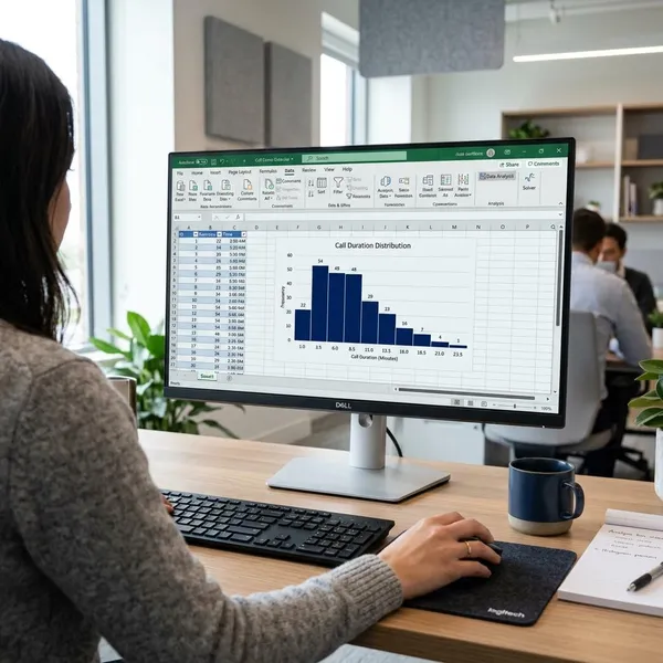
How to create a histogram with the Analysis ToolPak
Use the Analysis ToolPak method if your Excel version does not offer the built-in Histogram chart or if you want Excel to create a frequency table at the same time. It takes a few more steps because you must provide the bin limits yourself.
Enable the Analysis ToolPak
Go to File > Options > Add-ins. At the bottom, choose Excel Add-ins, click Go, check Analysis ToolPak, and select OK.
After it is enabled, the Data Analysis button should appear on the Data tab. If you are using Excel in a locked-down work or school environment, you may need permission to enable add-ins.
Enter bin upper limits in a separate column
Create a separate column with the upper limit for each bin. If you want bins ending at 10, 20, 30, and 40, enter those numbers in ascending order.
Think of these as cutoff points, not labels. Excel will count how many values fall up to each limit, so messy or out-of-order bin limits can produce confusing output.
Open Data > Data Analysis > Histogram
Go to Data, click Data Analysis, choose Histogram, and click OK. This opens the setup window for the ToolPak histogram.
Select the input and bin ranges
In Input Range, select the original numeric data. In Bin Range, select the separate bin-limit column you created.
- Check Labels if your selected ranges include headers.
- Use the same worksheet for quick testing.
- Use a new worksheet for cleaner report output.
Choose Chart Output and generate the results
Select Chart Output, choose where the results should appear, and click OK. Excel will generate a frequency table and a chart based on your bin limits.
One important difference: ToolPak results are often more static than a built-in chart. If the source data changes, expect to rerun the analysis rather than assuming everything updated automatically.
Conclusion
The simplest route is to clean one column of raw numbers, insert the built-in Histogram chart, and then adjust the bins until the distribution is easy to read. Use the ToolPak when the chart option is unavailable or when you need a frequency table, but do not skip the bin check; that is the step that turns the chart from a quick visual into something you can trust.